Parametric Equations
by Elizabeth Gieseking
Parametric equations are sets of equations in which the Cartesian coordinates are expressed as explicit functions of one or more parameters. For this exploration, we will be primarily considering equations of x and y as functions of a single parameter, t. The parameter, t, is often considered as time in the equation. Any equation that can be written in Cartesian or polar coordinates can also be written as a series of parametric equations, with the advantage of being able to view this relationship as it varies in time.
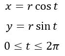
The first set of parametric equations we will consider will be the equation of a circle. In Cartesian coordinates, we write the equation as
In parametric equations, we have separate equations for x and y and we also have to consider the domain of our parameter. To draw a complete circle, we can use the following set of parametric equations.
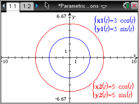
On handheld graphing calculators, parametric equations are usually entered as as a pair of equations in x and y as written above. The following graph is from a TI-nspire calculator.
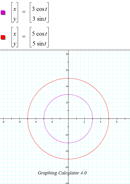
Computer based graphing programs have different methods of showing parametric equations. Graphing Calculator 4.0 shows parametric equations in a vector format and Desmos has users put the parameters directly into the coordinate pairs as shown below.
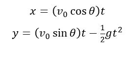
A traditional use of parametric equations is in physics, particulary when we wish to view two dimensional motion as a function of time. Consider the following equations for projectile motion.
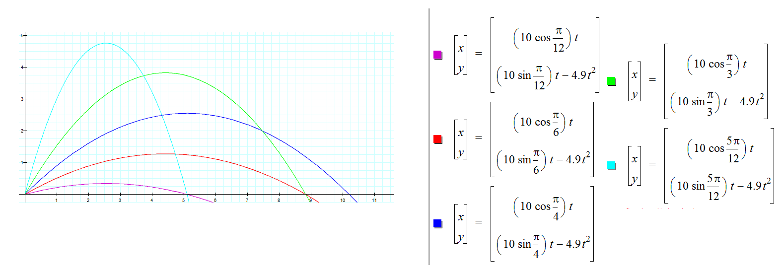
If we are given the magnitude and angle of the initial velocity, we can calculate the (x, y) coordinates as a function of time. The graph below shows the trajectories taken by an object with an inital velocity of 10 m/s and various launch angles. We can see both the maximum height that the projectile reaches and its range from this graph.
A more interesting use of these parametric equations is to actually watch the trajectory as a function of time. We will examine the same function, this time only considering the launch angle of
.
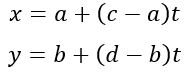
Parametric functions also give us a means of graphing lines and line segments. Let us assume we want to draw a segment from (a, b) to (c, d). We set our equations up as:
If we vary t from 0 to 1, our segment will start at (a, b) and end at (c, d). If we want to change the length of our segment, we can change the domain of t. For a true line,
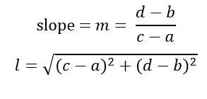
While this is impossible to actually graph, we can choose the domain of t such that our line extends the length of our screen. We can also calculate the slope and length of our segment.
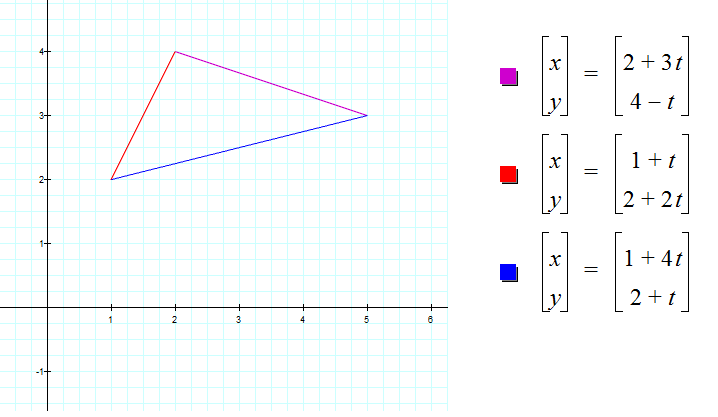
The following equations were used to graph a triangle as shown.
It was very easy to select the vertices of the triangles (2, 4), (1, 2), and (5, 3).
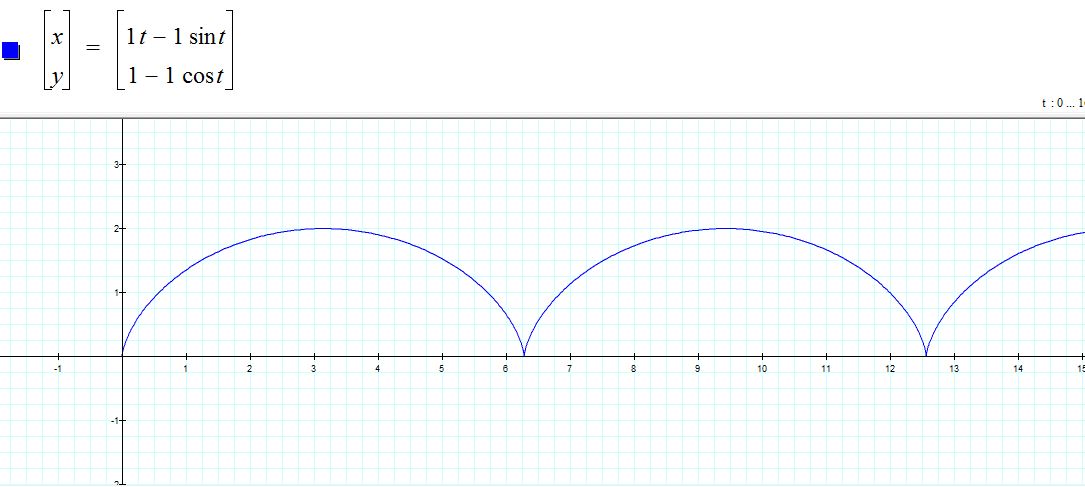
Although parametric equations can be used to graph circles and lines or segements, their real advantage comes when graphing relationships which are neither functions in rectangular nor polar coordinates. One such example is the cycloid. The cycloid is the path created when a given point along the circumference of a circle rolls along a line. The following cycloid is the graph created with a circle of radius 1 rolling along the x-axis.
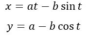
Related to the cycloid are the curtate cycloid and the prolate cycloid. Consider the equations
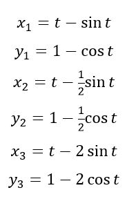
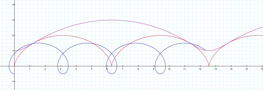
If a = b then we have a cycloid as shown above. If a > b then the point that is being traced is inside of the rolling circle and we have what is called a curtate cycloid. On the other hand, if a < b then the point that is being traced is outside of the rolling circle and the resulting curve is called a prolate cycloid. The following graph traces the movement for:
In the first set of parametric equations, a = b = 1, resulting in a cycloid, graphed in red. In the second set, a > b, resulting in a curtate cycloid, graphed in purple. In the third set of parametric equations, a < b, resulting in a prolate cycloid, graphed in blue. The moving circles associated with each cycloid are plotted in their corresponding colors. We see that the purple and blue circles are concentric with the red circle, corresponding to points inside and outside of the red circle.
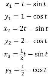
On these equations, we kept a constant at 1 and varied b. What happens when we keep b constant at 1 and vary a? We will examine the graph of the equations:
The first set of equations was unchanged. In the second set of parametric equations, a > b, again resulting in a curtate cycloid, graphed in purple. In the third set, a < b, again resulting in a prolate cycloid, graphed in blue.
We notice two major differences with this graph. First of all the cycle times are not the same length. In the time that the curtate cycloid completes one cycle, the cycloid completes two cycles, and the prolate cycloid completes 4 cycles. Secondly the amplitude of the prolate cycloid has decreased and the amplitude of the curtate cycloid has increased. We can better understand what is happening in these graphs if we look at the animation.
Looking at this graph, we see that when we change a, we are changing the radius of the rolling circle. The circles are rotating with a constant rotational velocity, so the larger circles are moving more quickly than the smaller circles. Also looking at the graph, we see that our second variable, b, corresponds to the distance from the center of the ball to the path being traced. In this case b was kept constant at 1. Thus we see that in our cycloid equations:
a is the radius of the circle moving along the x-axis and b is the distance of the point being traced from the center of the circle. Hence, when a = b, the point being traced is on the edge of the circle, when a > b, the point being traced is on the interior of the circle resulting in a curtate cycloid, and when a < b, the point being traced is outside the circle, resulting in a prolate cycloid.
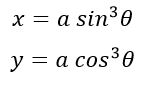
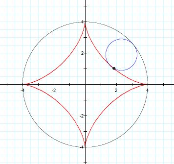
A curve that is similar to a cycloid is the hypocycloid of four cusps given by the parametric equations:
The hypocycloid is the path traced by a given point on a circle of radius a/4 as it rolls along inside a circle of radius a.
In this graph, a = 4, so the radius of the large circle is 4 and the radius of the small circle is 1. The small circle is given by the equation
. Below is an animation of this hypocycloid of four cusps.
From this exploration, we see that parametric equations have a number of benefits, including:
- The ability to see motion as a function of time
- The ability to easily define segments
- The ability to graph relations that are not functions in either rectangular or polar coordinates
Return to Elizabeth's Home Page